11 Categorical variables
A variable describing e.g. fuel consumption (or the height of a research patient) on a continuous scale is a continuous variable. Contrary to this, the hypothetical variable hypertension, which was introduced in chapter 9 and received either the value 0 or 1, is a categorical variable. More specifically, such dichotomous or binary variables, receiving most often either 0 or 1 as their values, are called dummy variables.
It is generally wise to tell R which of your variables are categorical variables so that R doesn’t mistakenly treat them as continuous variables in any analyses. In R, categorical variables should be saved as factor type. This is very easy.
You can view your data by typing the following command in the Console:
car_dataset5Even a quick glance at the output (only 4 lines are shown below) will reveal you that gear is meant to be a categorical variable in these data. The other variables are clearly continuous variables.
##                   fuel_cons_eu horsepower_eu  mass_eu gear
## Mazda RX4             11.20000      111.5279 1188.432    1
## Mazda RX4 Wag         11.20000      111.5279 1304.100    1
## Hornet Sportabout     12.57754      177.4308 1560.384    0
## Duster 360            16.44755      248.4031 1619.352    0
11.1 as.factor command
Let’s change the variable gear to factor, i.e. turn it into a categorical variable. We will save it over itself - we will not create a new dataset. There are a few easy ways to do this.
- option: With Base-R, the following would be done:
car_dataset5$gear <- as.factor(car_dataset5$gear)Note that in the expression car_dataset5$gear we indicate with the dollar sign $ that we want to change only the variable gear from the dataset car_dataset5 into factor.
- option is to do the same thing using dplyr:
car_dataset5 <- car_dataset5 %>% mutate(gear = as.factor(gear))Run either of the methods mentioned above. If you now look at your data again by typing the following command in the Console, you will not really see any difference from before (only 4 lines shown here):
car_dataset5## fuel_cons_eu horsepower_eu mass_eu gear
## Mazda RX4 11.20000 111.5279 1188.432 1
## Mazda RX4 Wag 11.20000 111.5279 1304.100 1
## Hornet Sportabout 12.57754 177.4308 1560.384 0
## Duster 360 16.44755 248.4031 1619.352 0Indeed, it is problematic that you can’t see in that output if R knows whether the variables are continuous or categorical.
tibble comes to the rescue. tibble is an improved version of the Base-R’s “dataframe” (in the previous examples, “car_dataset”, “car_dataset2” etc. were in Base-R format). At this point, tou don’t need to understand anything about data frames or why tibble is a better format - just take my word for it.
11.2 tibble
Let’s change our dataset “car_dataset5” into a tibble. Let’s save the new data set as “car_dataset6”.
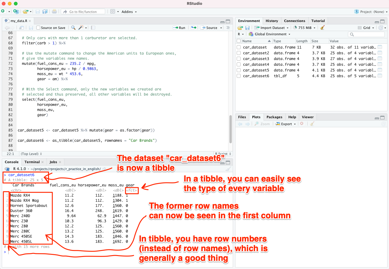
At the same time, we are making another important correction. So far, the rows in our dataset have been named after car brands, but naming rows in general is not recommended today. When we switch to the tibble format, line names are destroyed and replaced by line numbers. Car brands (or analogously: “code identifiers of participants”) will appear in the first column, which is a better practice.
It works like this - and notice that the command is nowadays as_tibble and not as.tibble:
car_dataset6 <- as_tibble(car_dataset5, rownames = "Car Brands")
After that, when you type the following command into the console, you can easily see that R indeed knows that the variable gear is categorical (or, in R’s terms, a factor):
car_dataset6
Below you can see 4 lines of data (see also the image below):
## # A tibble: 4 x 5
##   `Car Brands`      fuel_cons_eu horsepower_eu mass_eu gear
##   <chr>                    <dbl>         <dbl>   <dbl> <fct>
## 1 Mazda RX4                 11.2          112.   1188. 1
## 2 Mazda RX4 Wag             11.2          112.   1304. 1
## 3 Hornet Sportabout         12.6          177.   1560. 0
## 4 Duster 360                16.4          248.   1619. 0
R guide by Ville Langén is licensed under Attribution-ShareAlike 4.0 International